

Developing a plasma etch process has traditionally been an exercise in expert intuition combined with painstaking experimentation. A typical ICP-RIE process has 6–10 independently adjustable parameters — ICP power, bias power, pressure, gas flows, temperature, and more — creating a vast parameter space that is impractical to explore exhaustively. Researchers often rely on one-factor-at-a-time (OFAT) experiments or design-of-experiments (DOE) approaches, but both have significant limitations when dealing with complex, nonlinear process interactions.
Machine learning (ML) and artificial intelligence (AI) are changing this landscape. From accelerating recipe development to enabling real-time process control, data-driven approaches are making plasma etching smarter, faster, and more predictable. This article explores how ML is being applied to plasma etch processes, what tools and methods are most relevant for research labs, and how these approaches can enhance your existing workflow.
Why Plasma Etching Is Ripe for Machine Learning
Several characteristics of plasma etch processes make them particularly well-suited for ML approaches:
High dimensionality: With many interacting process parameters, the relationship between inputs (recipe settings) and outputs (etch rate, selectivity, profile angle, uniformity, surface roughness) is inherently multivariate and nonlinear. ML models excel at capturing these complex relationships.
Data-rich environment: Modern etch tools generate extensive process data — RF power readings, pressure traces, gas flow logs, optical emission spectra, and endpoint signals. This data is often logged but underutilized. ML transforms this data into actionable process intelligence.
Expensive experiments: Each etch run consumes materials, time, and tool capacity. ML can reduce the number of experiments needed to find an optimal process by intelligently selecting the most informative experiments to run.
Reproducibility challenges: Plasma processes can drift over time due to chamber conditioning, electrode and chamber-component aging, and polymer accumulation on the walls. ML models trained on process data can detect and compensate for these drifts before they cause yield loss.
Key Applications of ML in Plasma Etching
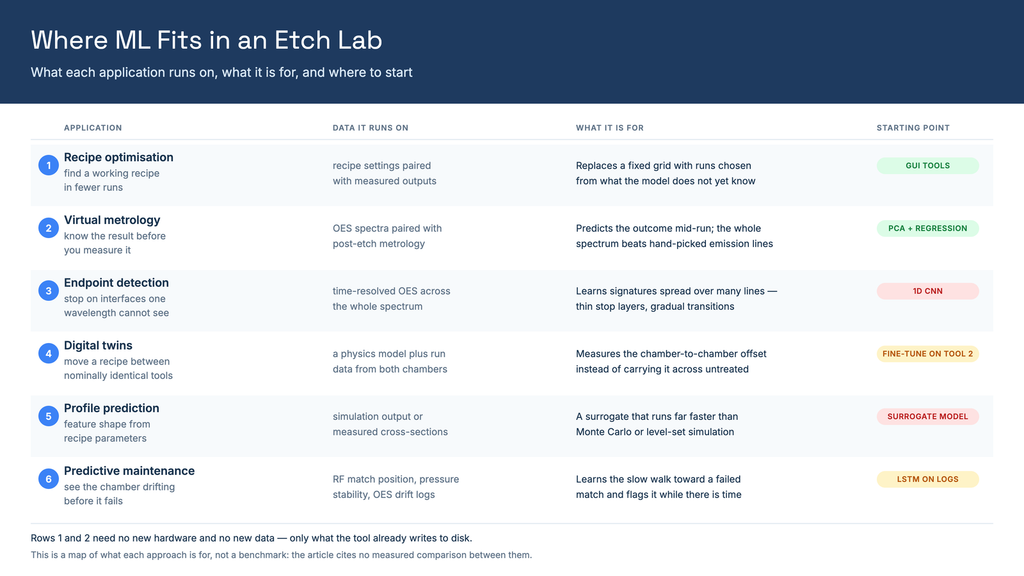
1. Process Recipe Optimization
The most immediate application is using ML to find optimal etch recipes faster than traditional DOE approaches. The workflow typically involves:
Data collection: Run an initial set of experiments (20–50 runs) spanning the parameter space of interest. Measure key outputs for each run.
Model training: Train a regression model (Gaussian process, random forest, or neural network) to predict etch outputs from recipe inputs.
Optimization: Use the trained model to identify optimal operating points — either maximizing a single metric or finding the best trade-off among competing objectives (e.g., high etch rate vs. low damage).
Bayesian optimization is particularly powerful here. Instead of requiring a dense grid of experiments, it uses the ML model’s uncertainty estimates to suggest the next most informative experiment.
The clearest published evidence that this competes with expert intuition comes from Kanarik et al. in Nature, who set process engineers and algorithms against each other on the same process-development task and found that a human-first, algorithm-second sequence beat either working alone. Two limits on how far that result travels are worth stating plainly: the study ran in a virtual process development environment rather than a physical chamber, and it measured cost-to-target on that task rather than run counts for any specific etch. It establishes that the collaboration pattern is worth adopting. It does not tell you how many runs your campaign will take.
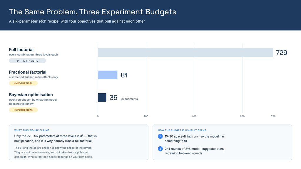
Illustrative Scenario — GaN HEMT Gate Recess: Consider optimising an ICP-RIE gate recess for GaN HEMTs across six recipe parameters, balancing etch rate, surface roughness, sidewall angle and nitrogen vacancy density. One part of this is arithmetic rather than assumption: a full factorial at three levels per parameter is 36 = 729 runs, which is why nobody runs one. Suppose a screened fractional design brings that to 81, and a Bayesian optimisation loop converges in 35. Those two numbers are hypothetical — chosen to show the shape of the saving, not taken from a published campaign. What a real loop would need, and what surface finish or profile it would land, depends on the measurement noise, how smooth the response surface turns out to be, and how sharply the four objectives conflict.
2. Virtual Metrology and Real-Time Prediction
Virtual metrology uses in-situ sensor data (optical emission spectroscopy, RF impedance, pressure readings) to predict etch outcomes in real time — without waiting for post-etch measurement.
By training ML models on paired datasets of sensor data and metrology results, researchers can:
- Predict etch rate and uniformity from OES spectral features during the etch
- Detect process excursions before they produce defective wafers
- Enable run-to-run control by adjusting recipe parameters based on real-time predictions
For research labs, the most accessible entry point is OES-based virtual metrology. Optical emission data is rich, high-dimensional, and readily available on most ICP and RIE systems. Principal component analysis (PCA) combined with simple regression models can provide surprisingly accurate real-time etch rate predictions.
Illustrative Scenario — OES-Based Virtual Metrology: Train a tree ensemble or a regularised regression on OES spectra paired with post-etch thickness measurements, and it can learn to predict remaining thickness while the run is still going. The transferable point is not a headline accuracy number but a structural one: giving the model the whole spectrum generally beats hand-picking a few emission lines, because the informative signal is spread across wavelengths that no single line captures. How close such a model gets to a standalone metrology tool is bounded by how repeatable that tool is on your own samples — measure that first, because it sets the ceiling.
3. Endpoint Detection Enhancement
Traditional endpoint detection relies on monitoring a single OES wavelength or reflectometry signal for a characteristic change when the etch reaches an interface. ML-enhanced endpoint detection uses the full OES spectrum (hundreds of wavelengths simultaneously) to detect more subtle transitions, such as:
- Thin etch-stop layers (< 5 nm)
- Compositional gradients rather than sharp interfaces
- Partial exposure of underlying layers in non-uniform processes
Algorithms like change-point detection, hidden Markov models, and convolutional neural networks applied to spectral time series can catch transitions that single-wavelength monitoring would miss.
Illustrative Scenario — Endpoint on a Thin Stop Layer: A one-dimensional convolutional network trained on time-resolved OES learns correlations spread across many emission lines rather than watching one, which is exactly what a thin high-k stop layer demands: the by-product signal is weak, the open area is small, and the transition is gradual rather than a step. That makes it the natural candidate where single-wavelength monitoring has already failed. Whether it works on your stack is an empirical question with a concrete test — check whether the model’s endpoint call agrees with a destructive cross-section on your own wafers before you trust it to stop a run.
4. Digital Twins of Etch Chambers
A digital twin is a computational model that mirrors the behavior of a physical etch chamber. It combines physics-based models (plasma kinetics, gas-phase transport, surface reactions) with ML models trained on experimental data to create a comprehensive simulation environment.
Digital twins enable:
- Virtual experimentation: Test new recipes computationally before running physical experiments
- Chamber matching: Understand and compensate for differences between nominally identical etch tools
- Predictive maintenance: Forecast when chamber components need replacement based on process drift patterns
- Transfer learning: Accelerate recipe development on a new tool by leveraging the digital twin from an existing, well-characterized system
Illustrative Scenario — Chamber Matching: Where a twin already exists for a well-characterised chamber, fine-tuning it on a modest set of runs from a second chamber is a better route to recipe transfer than copying setpoints across. Copying carries whatever chamber-to-chamber offset exists into the new tool untreated; fine-tuning at least measures it. Both the size of that offset and the improvement you get from correcting it are specific to the pair of chambers, so treat this as a method to try rather than a number to expect — and quantify your own baseline offset before deciding the effort is worth it.
5. Feature-Scale Profile Prediction
Predicting the 3D shape of etched features (trench profiles, via sidewalls, undercut geometry) from process parameters is one of the most challenging problems in etch modeling. Traditional feature-scale simulations (Monte Carlo methods, level-set methods) are computationally expensive and require detailed knowledge of surface reaction probabilities.
ML surrogate models trained on simulation data or experimental cross-sections can predict feature profiles orders of magnitude faster than physics-based simulations. This enables rapid exploration of how recipe changes affect feature geometry — particularly valuable for developing high-aspect-ratio etch processes.
6. Predictive Maintenance and Chamber Health Monitoring
Beyond process optimization, ML is proving valuable for predicting when etch chamber components will fail or degrade. By monitoring trends in process sensor data (RF reflected power, matching network positions, pressure stability, OES drift), ML models can forecast maintenance needs days or weeks in advance.
Illustrative Scenario — RF Match Degradation: A sequence model such as an LSTM, given a long enough history of RF matching-network positions, can learn what the slow walk toward a failed match looks like and raise a flag before the match actually fails. The appeal for a research lab is the input rather than the algorithm: this runs on log data the tool already writes, with no additional sensors to install. How much warning it buys, and what false-positive rate comes with that warning, depends on how much history you have and whether your particular failure mode creeps or arrives abruptly — a mode that fails without warning cannot be predicted from trend data at all.
ML Tool Guide for Research Labs
You don’t need a data science team to start applying ML to your etch processes:
Beginner Level (No ML Experience Required)
- JMP (SAS) — JMP Student Edition is free for eligible academic users; commercial subscriptions are priced separately: GUI-based DOE design, regression modeling, and visualization. The “Gaussian Process” platform is directly applicable to etch optimization. No programming required. Check current eligibility and pricing with SAS before budgeting.
- MATLAB Statistics and Machine Learning Toolbox: Familiar to most engineers. The
fitrgp(Gaussian process regression) andbayesopt(Bayesian optimization) functions are powerful and well-documented. - Google Colab — Free: Cloud-based Jupyter notebooks with Python + scikit-learn pre-installed. Good for trying out ML workflows before committing to a local installation.
Intermediate Level (Basic Python Familiarity)
- Python + scikit-learn — Free: The most versatile open-source ML library. Key functions:
GaussianProcessRegressor,RandomForestRegressor,cross_val_score. - BoTorch / Ax (Meta) — Free: State-of-the-art Bayesian optimization framework. Supports multi-objective optimization natively — ideal for balancing competing etch metrics.
- Optuna — Free: Lightweight optimization framework with automatic visualization of parameter importance and optimization history.
Advanced Level (ML/Data Science Background)
- PyTorch / TensorFlow — Free: For custom neural network models (virtual metrology, endpoint detection, profile prediction).
- Weights & Biases (wandb) — Free for academics: Experiment tracking platform for ML training runs.
- COMSOL Multiphysics + ML coupling: For physics-informed ML approaches. COMSOL’s plasma module can generate synthetic training data for feature-scale ML models.
A Step-by-Step Workflow for Your Lab
- Define your objective. What etch metrics matter most? Etch rate? Selectivity? Profile angle? Surface roughness? Define 2–3 key outputs to optimize.
- Identify variable parameters. Select 4–6 recipe parameters to vary. Keep other parameters fixed.
- Design initial experiments. Use a space-filling design (Latin hypercube or Sobol sequence) to place 15–30 initial experiments across the parameter space.
- Run experiments and measure. Execute the initial set. Record process sensor data (OES spectra, RF power/impedance, pressure traces) if available.
- Train initial model. Fit a Gaussian process or random forest model. Evaluate with leave-one-out cross-validation. If R² < 0.7, add more experiments or re-examine parameter ranges.
- Iterate with Bayesian optimization. Use the model to suggest the next 3–5 experiments. Run them, retrain, and repeat. Typically 2–4 iteration rounds suffice.
- Validate. Run 3–5 replicates at the predicted optimal conditions to verify predictions and assess process repeatability.
- Deploy and maintain. Periodically retrain with new data as chamber conditions evolve.
Data Management Best Practices
One of the biggest barriers to applying ML in research labs is not the algorithms — it is the data. Here are practical recommendations:
Structured Data Collection
Create a standardized data template for every etch run:
| Field | Example | Notes |
|---|---|---|
| Run ID | 2026-03-13-001 | Date + sequential number |
| Recipe name | SiO2_ICP_v3.2 | Version-controlled recipe |
| ICP Power (W) | 600 | Actual measured, not setpoint |
| Pressure (mTorr) | 15 | Actual measured average |
| Gas flows (sccm) | CF₄: 45, O₂: 5 | All gases |
| Etch rate (nm/min) | 185 | Method: ellipsometry |
| Uniformity (%) | 2.8 | 1σ, 49-point map |
| Wafers since clean | 15 | Chamber conditioning state |
Common Data Pitfalls
- Missing chamber state data: Always record wafers-since-clean, RF-on hours, and recent maintenance. Chamber condition is the #1 hidden variable that causes model degradation.
- Inconsistent metrology: If one researcher uses 5-point ellipsometry maps and another uses 49-point maps, the uniformity data is not comparable. Standardize measurement protocols.
- Setpoint vs. actual values: Always record actual measured values from tool logs, not recipe setpoints. A recipe calling for 600 W ICP power may deliver 585 W.
- Unlabeled process changes: If you changed the gas bottle, replaced an electrode, or performed maintenance, record it. These events create discontinuities that confuse ML models.
Worked Example: Bayesian Optimization of SiO₂ Etch
Problem Setup
Suppose you need to optimize an ICP-RIE process for SiO₂ etching. Your target metrics are: etch rate > 200 nm/min, uniformity < 3% (1σ), and selectivity to Si > 10:1. Variable parameters: ICP power (300–800 W), bias power (50–200 W), pressure (5–30 mTorr), and CF₄ flow (20–80 sccm), with O₂ flow fixed at 5 sccm and chuck temperature at 20°C.
Step 1: Initial Experiment Design
SciPy ships a Latin hypercube sampler, so this needs no extra DOE package. (Avoid pyDOE2 — it imports the imp module, which was removed in Python 3.12, so it fails on import there.)
# Space-filling initial design, using SciPy's quasi-Monte Carlo module
import numpy as np
import pandas as pd
from scipy.stats import qmc

RANDOM_SEED = 0

# (low, high, rounding step) — the step is what the tool will accept
DESIGN_SPACE = {
    "ICP_power":  (300, 800, 10),   # W
    "Bias_power": (50, 200, 10),    # W
    "Pressure":   (5, 30, 1),       # mTorr
    "CF4_flow":   (20, 80, 1),      # sccm
}

sampler = qmc.LatinHypercube(d=len(DESIGN_SPACE), seed=RANDOM_SEED)
design = sampler.random(n=20)

d_lo   = np.array([v[0] for v in DESIGN_SPACE.values()], dtype=float)
d_hi   = np.array([v[1] for v in DESIGN_SPACE.values()], dtype=float)
d_step = np.array([v[2] for v in DESIGN_SPACE.values()], dtype=float)

# Scale to real units, then round to what the tool will actually accept
scaled = qmc.scale(design, d_lo, d_hi)
experiments = pd.DataFrame(np.round(scaled / d_step) * d_step,
                           columns=list(DESIGN_SPACE))

print(experiments.head().to_string(index=False))
print(f"\n{len(experiments)} runs; discrepancy "
      f"{qmc.discrepancy(design):.4f} (lower is more evenly spread)")
Step 2: Load the Runs and Normalise the Inputs
Twenty completed runs, one row each. These values are hypothetical, generated for this example — they are not tool settings and must not be run as a recipe. Substitute your own CSV and the rest of the code is unchanged.
import numpy as np
import pandas as pd
from io import StringIO

RANDOM_SEED = 0   # fixed, so this example reproduces exactly

# In practice: runs = pd.read_csv("etch_runs.csv")
CSV = """ICP_power,Bias_power,Pressure,CF4_flow,etch_rate,uniformity,selectivity
500,160,7,22,167,6.4,8.2
370,70,29,25,108,5.2,14.9
580,70,27,74,197,3.8,15.4
690,130,14,33,218,4.2,10.2
610,110,19,59,212,3.7,12.2
450,100,17,48,157,2.9,12.7
560,190,12,77,237,4.9,7.3
740,140,5,76,253,5.9,8.8
720,90,23,28,210,4.6,13.4
640,150,20,71,235,3.6,9.9
800,160,8,68,272,5.6,8.1
770,130,29,41,225,5.8,11.6
520,80,22,47,178,3.2,14.5
350,60,16,62,136,2.6,15.2
660,190,24,61,246,5.6,8.6
380,110,26,54,141,4.8,12.9
450,120,10,29,145,5.0,10.5
410,180,13,36,158,5.5,8.9
540,170,18,52,201,4.0,9.6
320,50,11,39,107,3.6,14.9
"""
runs = pd.read_csv(StringIO(CSV))

PARAMS = {                      # name: (low, high, unit)
    "ICP_power":  (300, 800, "W"),
    "Bias_power": (50, 200, "W"),
    "Pressure":   (5, 30, "mTorr"),
    "CF4_flow":   (20, 80, "sccm"),
}
TARGETS = {"etch_rate": 200.0, "uniformity": 3.0, "selectivity": 10.0}

# Normalise to the unit cube so one length scale is meaningful across
# parameters measured in watts, millitorr and sccm.
lo = np.array([v[0] for v in PARAMS.values()], dtype=float)
hi = np.array([v[1] for v in PARAMS.values()], dtype=float)

def to_unit(X_real):
    return (np.asarray(X_real, dtype=float) - lo) / (hi - lo)

def to_real(X_unit):
    return np.asarray(X_unit, dtype=float) * (hi - lo) + lo

X      = to_unit(runs[list(PARAMS)].to_numpy())
y_rate = runs["etch_rate"].to_numpy(dtype=float)
y_unif = runs["uniformity"].to_numpy(dtype=float)
y_sel  = runs["selectivity"].to_numpy(dtype=float)
Step 3: Fit One Model per Response
The problem has three requirements, so it needs three models. A single model of etch rate cannot tell you whether a fast recipe also passes uniformity and selectivity.
from sklearn.gaussian_process import GaussianProcessRegressor
from sklearn.gaussian_process.kernels import Matern, ConstantKernel

# 1-sigma observation noise for each response, in its own units.
#
# Estimate it from replicates, not from a single repeat — one re-measurement
# gives you one difference and estimates nothing. Re-measuring the same wafer
# several times gives metrology repeatability; repeating the same recipe on
# several wafers gives the larger run-to-run figure, which also carries
# chamber drift. Use the run-to-run number here: the model is predicting what
# the next run will produce, not what the last wafer measured.
NOISE = {"etch_rate": 5.0, "uniformity": 0.2, "selectivity": 0.4}

def fit_gp(X, y, sigma_meas):
    # One shared length scale, not one per parameter. With 20 runs in four
    # dimensions, per-parameter (ARD) length scales are over-parameterised:
    # the fit declares a dimension irrelevant long before the data justify it.
    kernel = (ConstantKernel(1.0, (1e-2, 1e3))
              * Matern(length_scale=0.5, nu=2.5,
                       length_scale_bounds=(0.05, 20.0)))
    gp = GaussianProcessRegressor(
        kernel=kernel,
        alpha=(sigma_meas / y.std()) ** 2,   # known noise, normalised units
        normalize_y=True,
        n_restarts_optimizer=10, random_state=RANDOM_SEED)
    return gp.fit(X, y)

gp_rate = fit_gp(X, y_rate, NOISE["etch_rate"])
gp_unif = fit_gp(X, y_unif, NOISE["uniformity"])
gp_sel  = fit_gp(X, y_sel,  NOISE["selectivity"])
Step 4: A Constraint-Aware Acquisition Function
Expected improvement alone chases etch rate and will happily recommend a recipe that fails the other two requirements. Multiplying it by the probability that each constraint holds weights the search toward the feasible region — it does not fence it in. A point with a high enough expected improvement can still be proposed at 50 % feasibility, and points outside the feasible region are never assigned zero, only a small weight. Read the returned probabilities before committing the run; they are the part that tells you how much of a gamble it is.
acquisition = EI(etch rate) × P(uniformity < 3%) × P(selectivity > 10:1)
from scipy.stats import norm

EPS = 1e-9   # guards every division by a predictive standard deviation

def _predict(gp, x):
    mu, sd = gp.predict(np.atleast_2d(x), return_std=True)
    return float(mu[0]), max(float(sd[0]), EPS)

def expected_improvement(x, gp, y_best, xi=0.01):
    mu, sd = _predict(gp, x)
    imp = mu - y_best - xi
    z = imp / sd
    return imp * norm.cdf(z) + sd * norm.pdf(z)

def prob_below(gp, x, limit):
    mu, sd = _predict(gp, x)
    return float(norm.cdf((limit - mu) / sd))

def prob_above(gp, x, limit):
    mu, sd = _predict(gp, x)
    return float(norm.sf((limit - mu) / sd))

feasible = (y_unif < TARGETS["uniformity"]) & (y_sel > TARGETS["selectivity"])
HAS_FEASIBLE = bool(feasible.any())

# Improve on the best run that met BOTH constraints — not the fastest run
# overall, which may be infeasible.
y_best = float(y_rate[feasible].max()) if HAS_FEASIBLE else None

def acquisition(x):
    """Returns a scalar, negated because differential_evolution minimises."""
    p_unif = prob_below(gp_unif, x, TARGETS["uniformity"])
    p_sel  = prob_above(gp_sel,  x, TARGETS["selectivity"])
    if not HAS_FEASIBLE:
        # Nothing has satisfied the constraints yet, so there is no rate to
        # improve on. Hunt for a feasible point first; chasing rate now would
        # push the search further from the region you actually need.
        return -float(p_unif * p_sel)
    ei = expected_improvement(x, gp_rate, y_best)
    return -float(ei * p_unif * p_sel)
Step 5: Pick the Next Run and Convert Back to Tool Units
The optimiser works in the unit cube; the tool takes watts, millitorr and sccm. Converting back — and rounding to the resolution the tool actually accepts — is part of the loop, not an afterthought.
from scipy.optimize import differential_evolution

result = differential_evolution(
    acquisition, bounds=[(0.0, 1.0)] * X.shape[1],
    seed=RANDOM_SEED, tol=1e-6, polish=True)

# Round to the resolution the tool accepts, then evaluate the models at the
# recipe you will actually run — not at the optimiser's unrounded answer.
# Rounding moves the point, and at a borderline constraint that shift is
# large enough to change the reported probability.
STEP = np.array([10.0 if unit == "W" else 1.0
                 for (_, _, unit) in PARAMS.values()])
x_next = np.round(to_real(result.x) / STEP) * STEP
x_eval = to_unit(x_next)

if HAS_FEASIBLE:
    print(f"Feasible runs so far: {int(feasible.sum())} of {len(runs)}"
          f"   best feasible etch rate: {y_best:.0f} nm/min\n")
else:
    print(f"No feasible run in {len(runs)} yet — searching for one first\n")

print("Suggested next run")
for (name, (_, _, unit)), value in zip(PARAMS.items(), x_next):
    print(f"  {name:11s} {value:6.0f} {unit}")

print("\nModel expectation at that recipe (not a measurement)")
for label, gp, unit in (("etch rate", gp_rate, "nm/min"),
                        ("uniformity", gp_unif, "%"),
                        ("selectivity", gp_sel, ":1")):
    mu, sd = _predict(gp, x_eval)
    print(f"  {label:11s} {mu:7.2f} ± {sd:.2f} {unit}")

# Read these before committing the run — they are the feasibility gamble.
print(f"\n  P(uniformity < {TARGETS['uniformity']}%)    "
      f"{prob_below(gp_unif, x_eval, TARGETS['uniformity']):.2f}")
print(f"  P(selectivity > {TARGETS['selectivity']}:1)   "
      f"{prob_above(gp_sel, x_eval, TARGETS['selectivity']):.2f}")
What the Code Prints
This is the actual output of the code above, on the hypothetical data above. The recipe it suggests is a suggestion about where to run next, not a validated process:
Feasible runs so far: 2 of 20   best feasible etch rate: 157 nm/min

Suggested next run
  ICP_power      540 W
  Bias_power      80 W
  Pressure        17 mTorr
  CF4_flow        58 sccm

Model expectation at that recipe (not a measurement)
  etch rate    185.48 ± 2.91 nm/min
  uniformity     2.98 ± 0.51 %
  selectivity   13.72 ± 0.19 :1

  P(uniformity < 3.0%)    0.52
  P(selectivity > 10.0:1)   1.00
Two details in that output are worth dwelling on, because both are easy to get wrong.
The predictions are evaluated at the rounded recipe — 540 W, not the optimiser's 538.6 W. Reporting the model's opinion of a point you are not going to run is a small dishonesty that matters here: rounding to tool resolution shifts predicted uniformity from 2.96 % to 2.98 %, and the probability of passing a 3 % limit from 0.53 to 0.52. On a binding constraint, that is the difference you are actually taking a bet on.
And if no run in your data has yet satisfied both constraints, there is no feasible etch rate to improve on, so the code drops the improvement term and searches on feasibility alone until it finds one. Substituting a stricter uniformity limit into the same twenty rows shows the switch: the header becomes No feasible run in 20 yet — searching for one first, and the suggested recipe backs off from 185 nm/min to about 159 nm/min, trading rate for a chance at the feasible region. That is the correct move at that stage, and a loop that chased rate instead would walk away from it.
Why the Constraints Have to Be in the Acquisition Function
Delete the two probability terms — optimise etch rate alone, as a single-objective example would — and the same models on the same data recommend somewhere completely different:
| Acquisition | Suggested run | Predicted rate | Uniformity < 3% | Selectivity > 10:1 |
|---|---|---|---|---|
| EI on etch rate only | 800 W, 200 W, 14 mTorr, 80 sccm | 291 nm/min | 5.12 ± 0.85% — P(pass) < 0.01 | 6.66 ± 0.39:1 — P(pass) < 0.01 |
| EI × P(uniformity) × P(selectivity) | 540 W, 80 W, 17 mTorr, 58 sccm | 185 nm/min | 2.98 ± 0.51% — borderline, P(pass) = 0.52 | 13.72 ± 0.19:1 — P(pass) > 0.99 |
The unconstrained answer is faster and useless: it drives bias power to the top of its range, which is exactly what wrecks uniformity and selectivity.
The second row is what the code above prints. To reproduce the first, swap the acquisition function for one that ignores the constraints and re-run the same optimiser:
# The single-objective version, for comparison only — do not optimise this way
def unconstrained(x):
    return -expected_improvement(x, gp_rate, float(y_rate.max()))

worse = differential_evolution(
    unconstrained, bounds=[(0.0, 1.0)] * X.shape[1],
    seed=RANDOM_SEED, tol=1e-6, polish=True)

# Same rounding discipline as above: evaluate at the recipe you would run
w_eval = to_unit(np.round(to_real(worse.x) / STEP) * STEP)

for label, gp in (("etch rate", gp_rate), ("uniformity", gp_unif),
                  ("selectivity", gp_sel)):
    mu, sd = _predict(gp, w_eval)
    print(f"  {label:11s} {mu:7.2f} ± {sd:.2f}")
print(f"  P(uniformity < 3%)   {prob_below(gp_unif, w_eval, 3.0):.2f}")
print(f"  P(selectivity > 10)  {prob_above(gp_sel,  w_eval, 10.0):.2f}")
Both rows then come from the same twenty runs and the same three models — the only difference is whether the constraints are in the acquisition function.
Note also what the constrained run does not claim. Its predicted rate of 185 nm/min is below the 200 nm/min target, and the probability of meeting the uniformity limit is only about even. That is the honest state of the search after twenty runs: the model has found the feasible region but not yet a point inside it that also hits the rate target. The next few iterations are what close that gap — and if they do not, the constraint set may simply be infeasible on this tool, which is itself a useful finding.
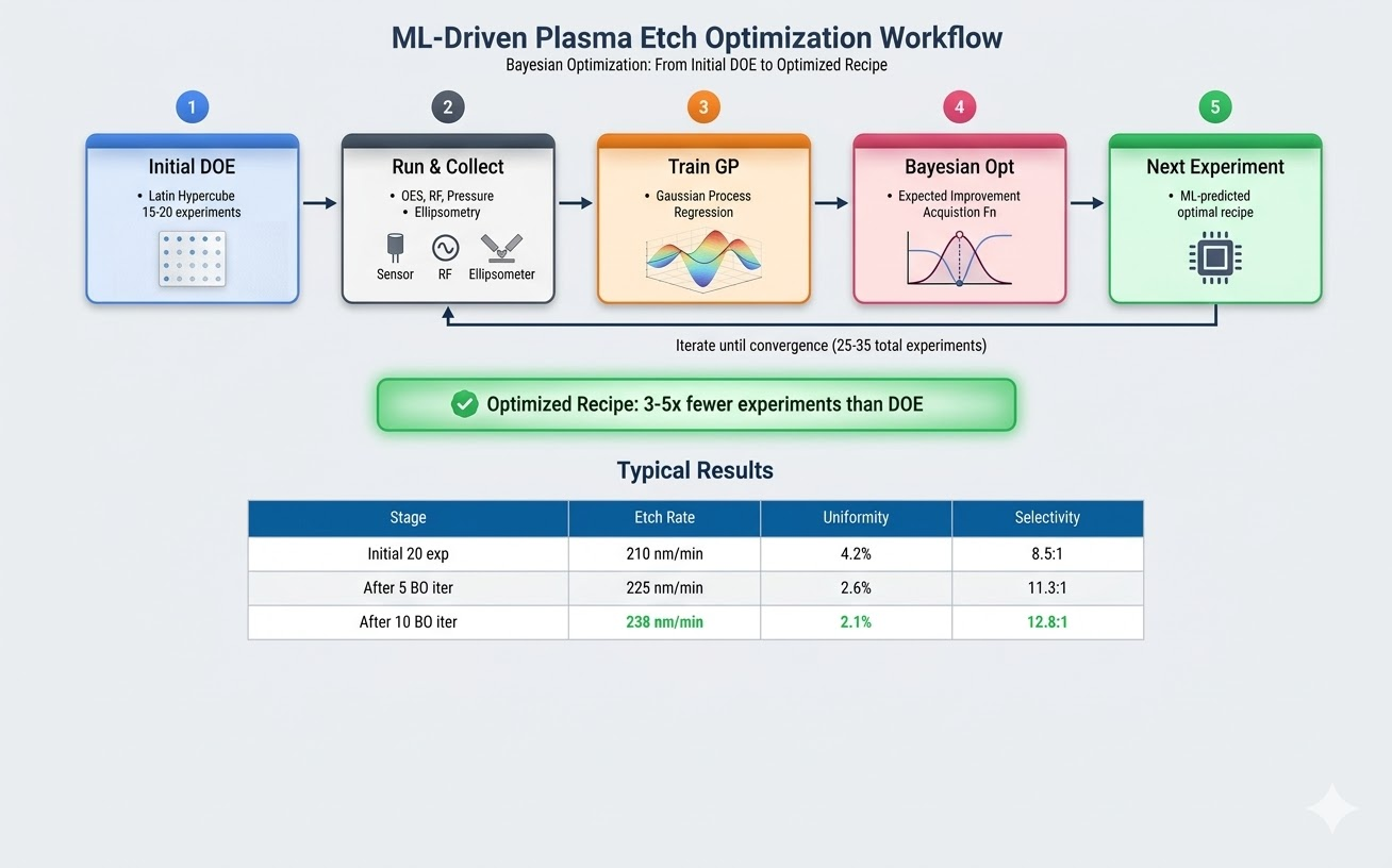
Figure 3: ML-Driven Etch Optimization Workflow — from initial experimental design through Bayesian optimization to validated recipes
Challenges and Limitations
Data quality matters more than data quantity. A small dataset with accurate, well-controlled measurements is far more valuable than a large dataset with inconsistent metrology. Before applying ML, ensure your measurement repeatability is adequate.
ML models are interpolators, not extrapolators. They work well within the parameter range covered by training data but can produce unreliable predictions outside that range. Always validate predictions that approach the boundaries of your experimental space.
Physical intuition remains essential. ML can identify optimal conditions, but understanding why a process works requires domain knowledge. Use ML as a complement to — not a replacement for — etch process fundamentals.
Chamber state variability. ML models trained on one chamber state may not generalize to a different state. Include chamber conditioning information in your dataset if possible.
Overfitting risk. With small datasets (< 30 points) and many parameters, overfitting is a real concern. Gaussian processes are often a good default for small-data etch optimisation because they return predictive uncertainty and regularise through the kernel and noise model rather than through a separate penalty term. That is not immunity: a badly chosen kernel, a length scale driven too short, a noise term estimated from too few repeats, or bounds that let a hyperparameter run to its limit will all produce a model that fits the training runs and misleads you everywhere else. Check kernel choice, cross-validated residuals and whether the predicted uncertainty is actually calibrated against repeat runs.
The Road Ahead
Automated experimentation: Closed-loop systems where ML algorithms design experiments, execute them on the tool, measure results, and iterate — all with minimal human intervention. The promise of these “self-driving labs” is compressing the time from a new material to a working recipe, though how much depends on where the current bottleneck sits: a lab limited by metrology turnaround gains more than one limited by tool availability.
Physics-informed ML: Hybrid models that embed known physics (e.g., Arrhenius rate dependencies, sheath models, ion angular distributions) as constraints within ML frameworks. These models require less training data and generalize better than pure data-driven approaches.
Federated learning across tools: ML models trained on data from multiple etch chambers, potentially across different labs, without sharing raw data.
Foundation models for semiconductor processing: Large-scale models pre-trained on diverse process data that can be fine-tuned for specific etch applications with minimal additional data.
ML-guided ALE development: Applying Bayesian optimization specifically to the challenging parameter space of atomic layer etching could significantly accelerate ALE recipe development for new materials. See our related article: Atomic Layer Etching (ALE): A Practical Guide for Research and Development.
Self-Driving Laboratories
The concept of a “self-driving lab” — where an ML algorithm designs experiments, an automated system executes them, and the results feed back into the model without human intervention — is an active area of work rather than a finished capability. The building blocks are individually mature: Bayesian optimization engines, automated wafer handling, and inline metrology that returns a number without breaking vacuum. Coupling them end to end on an etch tool is the part still being worked out.
For research labs, the practical first step is automating the loop rather than the lab: have the model suggest the next experiment, generate the recipe file, and import the metrology result after the run, with a person still loading wafers and sanity-checking each suggestion before it runs. Most of what this saves comes from removing the gap between a run finishing and someone deciding what to run next — so the payoff scales with how long that gap currently is in your lab, which is worth timing before you invest in closing it.
Conclusion
Machine learning is no longer a distant promise for plasma etch process development — it is a practical tool that can deliver immediate value in research labs. By reducing the number of experiments needed for recipe optimization, enabling real-time process monitoring, and providing predictive capability that traditional approaches cannot match, ML helps researchers spend less time on trial-and-error and more time on the science that matters.
NineScrolls’ etching and deposition systems are designed with comprehensive process data logging and diagnostic capabilities, providing the foundation for data-driven process optimization. Contact us to learn how our systems can support your smart manufacturing research.
Related Articles in This Series
- Atomic Layer Etching (ALE) — precision etching where ML-optimized recipes add significant value
- The Selectivity Challenge — achieving ultra-high etch selectivity with data-driven optimization
- Etching Beyond Silicon — plasma processing challenges where ML accelerates recipe development
Frequently Asked Questions
How many experiments do I need to get started with ML-based etch optimization?
A common starting point is 15–20 well-designed runs from a Latin hypercube or Sobol sequence, which is usually enough to fit an initial Gaussian process and begin iterating. There is no universal total beyond that. How many runs a campaign needs depends on how many parameters you are varying, how noisy your measurements are, how smooth the response surface turns out to be, and how many constraints have to hold at once — a two-parameter problem with repeatable metrology behaves nothing like a six-parameter one with run-to-run drift. Budget by watching whether the model’s predictions and its uncertainty are still improving, rather than against a target count.
Do I need programming experience to use ML for etch optimization?
No. GUI-based tools like JMP (SAS) provide Gaussian process regression and DOE design without any programming. MATLAB’s bayesopt function requires only a few lines of code. For researchers comfortable with basic Python, scikit-learn and Google Colab (free, cloud-based) offer powerful ML capabilities with extensive tutorials.
What sensor data from my etch tool is most useful for ML?
Optical emission spectroscopy (OES) data is the most valuable — it provides hundreds of wavelength channels that capture real-time plasma chemistry information. RF power and impedance data, chamber pressure traces, and gas flow logs are also useful. The key is to start saving and organizing it systematically, including chamber state metadata like wafers-since-clean and maintenance history.
Can ML models transfer between different etch chambers?
Partly, through transfer learning. A model trained on one reference chamber can be fine-tuned on a modest set of runs from a second chamber, which is generally a better route than copying setpoints across — copying carries whatever offset exists between the two tools into the new one untreated, while fine-tuning at least measures it. How large that offset is, and how much fine-tuning closes it, is specific to your pair of chambers; measure your own baseline deviation before assuming the effort pays for itself.
What is the biggest mistake labs make when starting with ML for etch processes?
Poor data management. Etch process data is often scattered across tool logs, lab notebooks, and individual files with inconsistent formats. The most impactful first step is creating a standardized data template that records actual measured values (not setpoints), includes chamber conditioning state, and is consistently used by all researchers.
References and Further Reading
- Oehrlein, G. S., et al. “Future of plasma etching for microelectronics: Challenges and opportunities.” J. Vac. Sci. Technol. B 42, 041501 (2024). doi:10.1116/6.0003579
- Krüger, F., Zhang, D., Luan, P., Park, M., Metz, A., & Kushner, M. J. “Autonomous hybrid optimization of a SiO₂ plasma etching mechanism.” J. Vac. Sci. Technol. A 42, 043008 (2024). doi:10.1116/6.0003554
- Guo, J., Mou, Z., Ren, K., Ni, D., & Gao, D. “Sequence modeling for predicting three-dimensional plasma etching profiles with deep learning.” J. Vac. Sci. Technol. A 43, 043005 (2025). doi:10.1116/6.0004669
- Snoek, J., et al. “Practical Bayesian optimization of machine learning algorithms.” NeurIPS (2012).
- Kanarik, K. J., et al. “Human–machine collaboration for improving semiconductor process development.” Nature 616, 707 (2023).